Amuse-bouches from useR!2019

dplyr example

Let’s say you have a dataset, here iris, and you want to compute the average Petal.Length for each Species:

library(dplyr)

## 
## Attaching package: 'dplyr'

## The following objects are masked from 'package:stats':
## 
##     filter, lag

## The following objects are masked from 'package:base':
## 
##     intersect, setdiff, setequal, union

iris %>% 
  group_by(Species) %>%
  summarise(avg = mean(Petal.Length, na.rm = TRUE))

## # A tibble: 3 x 2
##   Species      avg
##   <fct>      <dbl>
## 1 setosa      1.46
## 2 versicolor  4.26
## 3 virginica   5.55

You can use the “curly-curly” brackets if you want to turn this small bit of code into a function group_mean() with a data, by and var argument² (and want to pass the variables on in an unquoted way):

group_mean <- function(data, by, var) {
  
  data %>%
    group_by({{ by }}) %>%
    summarise(avg = mean({{ var }}, na.rm = TRUE))
}

We can then apply group_mean() to any dataset that has a grouping and a continuous variable, for example, the mammals sleep dataset in ggplot2:

library(ggplot2)
group_mean(data = msleep, by = vore, var = sleep_total)

ggplot2 example

Another common tidy eval application is ggplot2. In the example below, we want a customised plot: a scatterplot with a geom_smooth on top of it.

library(ggplot2)
theme_set(theme_bw())
ggplot(data = iris, 
       aes(x = Sepal.Length, y = Petal.Length, group = Species, color = Species)
       ) +
  geom_point() +
  geom_smooth(method = "lm") + 
  ggtitle("Pack this plot into a function.")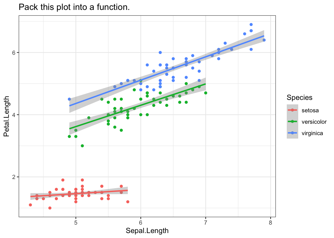

Again, we can wrap the “curly-curly” brackets around the arguments and apply them to a different dataset.

plot_point_smooth <- function(data, x, y, gr = NULL, method = "lm") {
  
  ggplot(data = data, 
         aes({{ x }}, {{ y }}, group = {{ gr }}, color = {{ gr }})
         ) +
    geom_point() +
    geom_smooth(method = method)
  
}

plot_point_smooth(msleep, x = sleep_total, y = sleep_rem, gr = NULL) + 
  ggtitle("Tidy eval with the msleep dataset")

Create a package

If you want to create a package, do the following (see also screencast):

## 1. create the package skeleton
create_package("~/tmp/mypackage")

## 2. use git
use_git()

## 3. add a license
use_mit_license()

## 4. run check
# install.packages("devtools")
devtools::check()

## 5. commit all files with git

## 6. set up git + github
use_github()
## will update the DESCRIPTION file

## 7. install the package
devtools::install()

## 8. add a rmarkdown readme file
use_readme_rmd()
## knit + commit + push

## 9. clean up if this was only a demo
## install.packages("fs")
## fs::dir_delete("~/tmp/mypackage")

Conventional package installation

Play around with usethis³ and see what happens:

pak::pkg_install("usethis")
pak::pkg_remove("usethis")
pak::pkg_install("r-lib/usethis")
pak::pkg_status("usethis")

Package installation for projects

First, create a project with usethis, then install R packages directly into the project.

usethis::create_project("~/tmp/test")

## check the directory
dir()

## initialise a dedicated R packages folder
pak:::proj_create()

## check the directory again
dir()

## check the DESCRIPTION file
readLines("DESCRIPTION")

## install usethis
pak:::proj_install("usethis")

## this installs dependencies into a private project library
readLines("DESCRIPTION")

## remove the project folder again
fs::dir_delete("~/tmp/test")

Get some large’ish data

First, we need some large dataset. To not burden our laptops too much⁶, we will go for some exome based GWAS results.

## Source: https://portals.broadinstitute.org/collaboration/giant/index.php/GIANT_consortium_data_files

path_to_file_1 <- "Height_AA_add_SV.txt.gz"
path_to_file_2 <- "BMI_African_American.fmt.gzip" 


## Height
download.file(
  "https://portals.broadinstitute.org/collaboration/giant/images/8/80/Height_AA_add_SV.txt.gz",
  path_to_file_1)

## BMI
download.file(
  "https://portals.broadinstitute.org/collaboration/giant/images/3/33/BMI_African_American.fmt.gzip",
  path_to_file_2)


## File size
## install.packages("fs")
fs::file_size(path_to_file_1)

## 4.39M

fs::file_size(path_to_file_2)

## 13.3M

The two datasets have a mix of characters, numbers and decimals⁷.

vroom vs DT

Here is how vroom works and a basic comparison to data.table::fread (I let you do the proper benchmarking yourself).

library(dplyr)

## With vroom
giant_vroom <- vroom::vroom(path_to_file_1)
giant_vroom_subset <- giant_vroom %>% select(CHR, POS) %>% filter(CHR == 1)

## The equivalent with data.table
giant_DT <- data.table::fread(path_to_file_1)
giant_DT_subset <- giant_DT %>% select(CHR, POS) %>% filter(CHR == 1)

col_select for the win

## Selecting columns
giant_vroom_select <- vroom::vroom(path_to_file_1, 
                                   col_select = list(SNPNAME, ends_with("_MAF")))
head(giant_vroom_select)

## Preventing columns from being imported
giant_vroom_remove <- vroom::vroom(path_to_file_1, 
                                   col_select = -ExAC_AFR_MAF)
head(giant_vroom_remove)

## Renaming on the fly
giant_vroom_rename <- vroom::vroom(path_to_file_1, 
                                   col_select = list(p = Pvalue, everything()))
head(giant_vroom_rename)

Combining multiple datasets

data_combined <- vroom::vroom( 
                    c(path_to_file_1, path_to_file_2), 
                    id = "path")
table(data_combined$path)

Matrices with base-r

Let’s look at an example of matrix operations in base-r⁹.

First, we want to add two matrices with similar dimensions:

mat_1 <- matrix(c(15, 10, 8, 6, 12, 9), byrow = FALSE, nrow = 2) 
mat_2 <- matrix(c(5, 2, 3), nrow = 1)

## broadcasting won't work ❌
mat_1 + mat_2

## Error in mat_1 + mat_2: non-conformable arrays

Next, we want to select one matrix column:

dim(mat_1[,2:3]) ## selecting two columns is fine

## [1] 2 2

## subsetting won't preserve the matrix class ❌
dim(mat_1[,1]) ## why not 2x1?

## NULL

length(mat_1[,1]) ## ah, it turned into a vector!

## [1] 2

dim(mat_1[,1, drop = FALSE]) ## but with drop = FALSE we can keep it a matrix

## [1] 2 1

Matrices with rray

Let’s do now the same task with rray.

library(rray)

(mat_1_rray <- rray(c(15, 10, 8, 6, 12, 9), dim = c(2, 3)))
(mat_2_rray <- rray(c(5, 2, 3), dim = c(1, 3)))

## Broadcasting works ✓
mat_1_rray + mat_2_rray

## Subsetting works ✓
dim(mat_1_rray[,2:3])
dim(mat_1_rray[,1])

## smart functions
mat_1_rray / rray_sum(mat_1_rray, axes = 1)
rray_bind(mat_1_rray, mat_2_rray, .axis = 1)
rray_bind(mat_1_rray, mat_2_rray, .axis = 2)