LD Part 1

Access precomputed LD

May 21, 2019 14 min read

Code Source Document

Goal
Two approaches
Our toy data
1A. A solution that works: ldlink from NIH
- LDproxy
- LDmatrix
1B. A solution that almost works: ensembl.org
2. Solutions that work half-through
- SNPsnap
- API provided by sph.umich
3. A solution that does not work
- rsnps::ld_search
Conclusion
Session Info

R-packages used:

library(httr)
library(jsonlite)
library(xml2)
library(ggplot2)
theme_set(theme_bw())
library(tibble)
library(tidyr)
library(magrittr)
library(glue)
library(purrr)
library(rsnps)
library(data.table)
library(janitor)
library(stringr)
library(rsnps)

The squared correlation between genetic markers is one way to estimate linkage disequilibrium (LD). LD has to be computed all the time - either for as an input for statistical methods or to summarise results.

However, accessing LD estimations quickly, for a specific population and in an automated way (e.g. with R) is suprisingly difficult.

In this blog post I am exploring how to do this efficiently.

Goal

At the end of this blog post, we want to know the genetic correlation between two or more markers in a specific human population, so that we can populate the locuszoom plot from the previous blog post with coloured dots.

For simplicity, I will use the terms correlation, squared correlation, r, r2 and LD interchangeably.

Two approaches

In principle, there are two ways of doing accessing LD:

Download (or access) the genetic data from which you want to estimate your correlations + calculate the correlations using some efficient approach.
Access precomputed LD estimations.

Approach	Advantages	Downsides	Useful when…
(1) Local computation of LD	LD matrix can be quickly updated to new reference panels	Requires large computation and storage space (e.g. 1000 Genomes is >100 few GB large).	i) LD for a large set of SNPs is needed ii) LD from non-standard reference panel is needed.
(2) Access precomputed LD	not need for large computation and storage space.	limited to certain small sets of markers, limited to possibly outdated reference panels.	LD for a small set of SNPs is needed

For now, I will focus on approach (2), and then explore approach (1) in a future blog post.

Spoiler: Using approach (2) does not get you far. It took me quite a while to gather all the solutions that are listed below, and yet there is not one perfect/ideal solution.

Our toy data

We will recycle the data from the previous blog post, where the focus was on extracting annotation using the package biomaRt. In this blog post, we will complete that locuszoom plot by adding the LD information.

## Data Source URL
url <- "https://portals.broadinstitute.org/collaboration/giant/images/2/21/BMI_All_ancestry.fmt.gzip"

## Import BMI summary statistics dat.bmi <- read_tsv(file = url) ##
## taking too long, let's use fread instead.

dat.bmi <- data.table::fread(url, verbose = FALSE)

## Rename some columns
dat.bmi <- dat.bmi %>% rename(SNP = SNPNAME, P = Pvalue)

## Extract region
dat.bmi.sel <- dat.bmi %>% slice(which.min(P))
dat.bmi.sel

## range region
range <- 5e+05
sel.chr <- dat.bmi.sel$CHR
sel.pos <- dat.bmi.sel$POS

data <- dat.bmi %>%
  filter(CHR == sel.chr, between(POS, sel.pos -
    range, sel.pos + range))

head(data)

(snp <- dat.bmi.sel$SNP)

What we are interested in is the LD between our top SNP rs1421085 and all other 82 SNPs nearby.

This dataset has positions on build GRCh37, while most databases are on build GRCh38 by now.

sm <- rsnps::ncbi_snp_summary(snp) %>% separate(chrpos, c("chr", "pos"))
sel.pos == as.numeric(sm$pos)

## [1] FALSE

Let’s quickly repeat what our primary goal is:

Extract the correlation between SNPs

without downloading any data,
fairly quick and
in R.

1A. A solution that works: ldlink from NIH

ldlink is a website provided by NIH to easily (and programmatically) request LD estimates in population groups.

LD is estimated from Phase 3 of the 1000 Genomes Project and super- and subpopulations can be selected.

There are different ways to access the LD estimations (e.g. LDpair, LDmatrix, LDproxy) and the same modules are also available through the API.

To access the API, you need to register for a token (takes a few seconds).

MYTOKEN <- "a_mix_of_numbers_and_characters"

Let’s look at two modules:

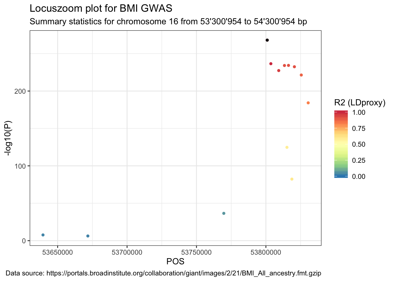
LDproxy: access LD between a SNP and its region
LDmatrix: access LD matrix

LDproxy

To get the LD between a SNP and its region.

First, access the API:

LDproxy_raw <- system(
  glue::glue("curl -k -X GET 'https://ldlink.nci.nih.gov/LDlinkRest/ldproxy?var={snp}&pop=EUR&r2_d=r2&token={MYTOKEN}'"),
  intern = TRUE
)

Then, do a bit of data wrangling to get a tidy data frame:

LDproxy <- LDproxy_raw %>%
  purrr::map(., function(x) stringr::str_split(x, "\t") %>%
      unlist()) %>% ## remove all the tabs
  do.call(rbind, .) %>% ## turn into a matrix
  data.frame() %>% ## turn into a data frame
  janitor::row_to_names(1) %>% ## make the first row the column names
  rename(SNP = RS_Number) %>% ## rename RS_Number as SNP
  mutate_at(vars(MAF:R2), function(x) as.numeric(as.character(x))) %>% ## turn MAF:R2 columns numeric
  mutate(SNP = as.character(SNP)) ## turn SNP from a factor into a character
head(LDproxy)

##          SNP          Coord Alleles    MAF Distance Dprime     R2
## 1  rs1421085 chr16:53800954   (T/C) 0.4324        0 1.0000 1.0000
## 2 rs11642015 chr16:53802494   (C/T) 0.4324     1540 1.0000 1.0000
## 3 rs62048402 chr16:53803223   (G/A) 0.4324     2269 1.0000 1.0000
## 4  rs1558902 chr16:53803574   (T/A) 0.4324     2620 1.0000 1.0000
## 5 rs55872725 chr16:53809123   (C/T) 0.4324     8169 1.0000 1.0000
## 6 rs56094641 chr16:53806453   (A/G) 0.4344     5499 0.9959 0.9839
##   Correlated_Alleles RegulomeDB Function
## 1            T=T,C=C          5       NA
## 2            T=C,C=T          4       NA
## 3            T=G,C=A          5       NA
## 4            T=T,C=A          7       NA
## 5            T=C,C=T          4       NA
## 6            T=A,C=G          6       NA

Next, join the original summary stats data with the LDproxy data frame.

data_ldproxy <- data %>%
  right_join(LDproxy, by = c("SNP" = "SNP"))

Lastly, plot the summary statistics with the point colour indicating the R2.

ggplot(data = data_ldproxy) +
  geom_point(aes(POS, -log10(P), color = R2), shape = 16) +
  labs(
    title = "Locuszoom plot for BMI GWAS",
    subtitle = paste(
      "Summary statistics for chromosome", sel.chr, "from",
      format((sel.pos - range), big.mark = "'"), "to",
      format((sel.pos + range), big.mark = "'"), "bp"
    ),
    caption = paste("Data source:", url)
  ) +
  geom_point(
    data = data_ldproxy %>% filter(SNP == snp),
    aes(POS, -log10(P)), color = "black", shape = 16
  ) +
  scale_color_distiller("R2 (LDproxy)",
    type = "div", palette = "Spectral",
    limits = c(0, 1)
  )

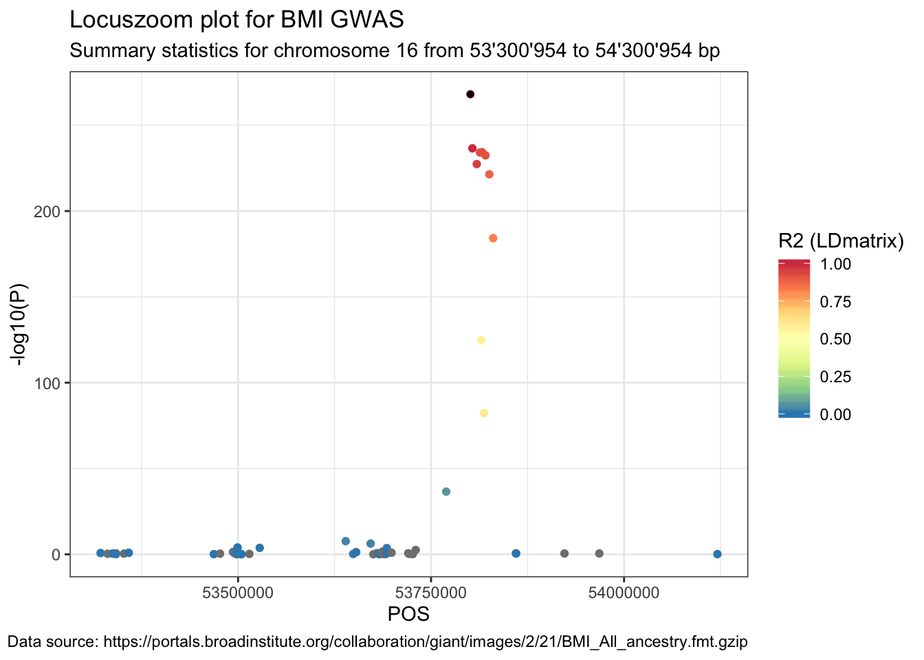
LDmatrix

LDmatrix module accesses the pairwise LD between a set of SNPs.

Again, first access the API:

snplist <- data %>%
  filter(str_detect(SNP, "rs")) %>%
  pull(SNP) %>%
  paste(collapse = "%0A")

LDmatrix_raw <- system(
  glue::glue("curl -k -X GET 'https://ldlink.nci.nih.gov/LDlinkRest/ldmatrix?snps={snplist}&pop=CEU%2BTSI%2BFIN%2BGBR%2BIBS&r2_d=r2&token={MYTOKEN}'"),
  intern = TRUE
)

If you want to access the dprime (d’) values, write r2_d=d.
If you want to access certain sub populations, let’s say CEU, TSI and FIN, concatenate them with %B in between: CEU%2BTSI%2BFIN.

Then, do a little data tidying:

LDmatrix <- LDmatrix_raw %>%
  purrr::map(., function(x) stringr::str_split(x, "\t") %>%
      unlist()) %>%
  do.call(rbind, .) %>% ## turn into a matrix
  data.frame() %>% ## turn into a data.frame
  janitor::row_to_names(1) ## make the first line the column names

LDmatrix_long <- LDmatrix %>%
  gather("SNP2", "R2", -RS_number) %>% ## from wide to long
  rename(SNP = RS_number) %>% ## rename RS_number
  mutate(R2 = as.numeric(R2)) %>% ## make R2 numeric
  mutate_if(is.factor, as.character) ## make all factor columns characters

## Warning: attributes are not identical across measure variables;
## they will be dropped

## Warning: NAs introduced by coercion

head(LDmatrix_long)

##           SNP       SNP2    R2
## 1  rs61754093 rs61754093 1.000
## 2 rs181111349 rs61754093    NA
## 3 rs199662749 rs61754093    NA
## 4 rs189080082 rs61754093 0.000
## 5   rs6499548 rs61754093 0.023
## 6 rs139704369 rs61754093    NA

Next, join the original summary stats data with the LDmatrix_long data frame.

data_ldmatrix <- data %>%
  right_join(LDmatrix_long, by = c("SNP" = "SNP"))

Lastly, plot the summary statistics with the point colour indicating the R2.

ggplot(data = data_ldmatrix %>% filter(SNP2 == snp)) +
  geom_point(aes(POS, -log10(P), color = R2)) +
  labs(
    title = "Locuszoom plot for BMI GWAS",
    subtitle = paste(
      "Summary statistics for chromosome", sel.chr, "from",
      format((sel.pos - range), big.mark = "'"), "to",
      format((sel.pos + range), big.mark = "'"), "bp"
    ),
    caption = paste("Data source:", url)
  ) +
  geom_point(
    data = data_ldmatrix %>% filter(SNP == snp & SNP2 == snp),
    aes(POS, -log10(P)), color = "black", shape = 16
  ) +
  scale_color_distiller("R2 (LDmatrix)",
    type = "div", palette = "Spectral",
    limits = c(0, 1)
  )

1B. A solution that almost works: ensembl.org

The REST API of Ensembl can do a lot (see options here). For example access precomputed LD. The webpage even provides R code to do so, which is from where I copied some snippets below.

To access the rest API at ensembl, we need the following three packages loaded.

library(httr)
library(jsonlite)
library(xml2)

What reference panels/population can we choose from?

Currently, the largest and hence most popular public reference panel is 1000 Genomes reference panel (1KG). The 26 populations of roughly 100 individuals each can be grouped into five super populations: African (AFR), American (AMR), European (EUR), South Asian (SAS), East Asian (EAS).

We can ask the ENSEMBL API from what populations reference panels are available. This will return us a data frame.

server <- "https://rest.ensembl.org"
ext <- "/info/variation/populations/homo_sapiens?filter=LD"

r <- GET(paste(server, ext, sep = ""), content_type("application/json"))

stop_for_status(r)

head(fromJSON(toJSON(content(r))))

##                                                  description size
## 1                              African Caribbean in Barbados   96
## 2                           African Ancestry in Southwest US   61
## 3                                      Bengali in Bangladesh   86
## 4                        Chinese Dai in Xishuangbanna, China   93
## 5 Utah residents with Northern and Western European ancestry   99
## 6                               Han Chinese in Bejing, China  103
##                      name
## 1 1000GENOMES:phase_3:ACB
## 2 1000GENOMES:phase_3:ASW
## 3 1000GENOMES:phase_3:BEB
## 4 1000GENOMES:phase_3:CDX
## 5 1000GENOMES:phase_3:CEU
## 6 1000GENOMES:phase_3:CHB

name stands for the population identifier. size refers to the number of individuals in the reference panel. Note that these are all populations with around 100 individuals (the correlation estimation will have an error that scales with the sample size). There are also the five super population available (although not listed here), simply replace the last three characters in name by EUR, AFR, AMR, EAS, SAS.

^{(From this blog post.)}

We want the LD information, so that we can add this info to the locuszoom plot. But how do we know which population to pick? One way is to read up what kind of individuals were present. In our case - mostly Europeans (EUR). But we could also build some pooled LD matrix of different populations.

Now that we know which reference panel we want to use, we can use the different rest APIs.

Access LD between a SNP and its region
Access LD matrix
Access LD between a SNP and many other SNPs

Access LD between a SNP and its region

This API is described here.

The default window size is 500 kb. There are also thresholds for r2 (e.g. if you want to filter all SNPs with an r2 > 0.8).

The only input required is the SNP rsid, marked with {snp}.

snp

## [1] "rs1421085"

server <- "https://rest.ensembl.org"
ext <- glue::glue("/ld/human/{snp}/1000GENOMES:phase_3:EUR?")
## Window size in kb. The maximum allowed value for the window size is 500 kb. LD is computed for the given variant and all variants that are located within the specified window.

r <- GET(paste(server, ext, sep = ""), content_type("application/json"))
stop_for_status(r)
LD.SNP.region <- as_tibble(fromJSON(toJSON(content(r)))) %>%
  unnest() %>%
  mutate(r2 = as.numeric(r2))

## Warning: `cols` is now required.
## Please use `cols = c(variation1, d_prime, r2, population_name, variation2)`

head(LD.SNP.region)

## # A tibble: 6 x 5
##   variation1 d_prime      r2 population_name         variation2
##   <chr>      <chr>     <dbl> <chr>                   <chr>     
## 1 rs1421085  0.327013 0.0834 1000GENOMES:phase_3:EUR rs8043738 
## 2 rs1421085  0.992084 0.409  1000GENOMES:phase_3:EUR rs2042031 
## 3 rs1421085  0.846280 0.647  1000GENOMES:phase_3:EUR rs11642841
## 4 rs1421085  1.000000 0.957  1000GENOMES:phase_3:EUR rs9940128 
## 5 rs1421085  0.999948 0.0552 1000GENOMES:phase_3:EUR rs73612011
## 6 rs1421085  0.907868 0.648  1000GENOMES:phase_3:EUR rs8057044

As a result, LD.snp.region contains the r2 of our top SNP with all SNPs that were +/- 500 kb away.

What if we want the correlation between all SNPs?

Access LD matrix

For this, we need the rest API here.

We can calculate the LD matrix of a full region, max 1 Mb wide. For fast computation, we limit it to +/- 50 kb.

## Query region. A maximum of 1Mb is allowed.

ext <- glue::glue("/ld/human/region/{sel.chr}:{sel.pos - range/20}..{sel.pos + range/20}/1000GENOMES:phase_3:EUR?")

r <- GET(paste(server, ext, sep = ""), content_type("application/json"))
stop_for_status(r)
LD.matrix.region <- as_tibble(fromJSON(toJSON(content(r)))) %>%
  unnest() %>%
  mutate(r2 = as.numeric(r2))

## Warning: `cols` is now required.
## Please use `cols = c(population_name, r2, variation2, variation1, d_prime)`

head(LD.matrix.region)

## # A tibble: 6 x 5
##   population_name            r2 variation2  variation1 d_prime 
##   <chr>                   <dbl> <chr>       <chr>      <chr>   
## 1 1000GENOMES:phase_3:EUR 0.761 rs9933509   rs8057044  0.999998
## 2 1000GENOMES:phase_3:EUR 1     rs150763868 rs72803680 1.000000
## 3 1000GENOMES:phase_3:EUR 0.106 rs7206122   rs62033401 0.999940
## 4 1000GENOMES:phase_3:EUR 0.731 rs9935401   rs8057044  0.999997
## 5 1000GENOMES:phase_3:EUR 0.106 rs141816793 rs62033399 0.999943
## 6 1000GENOMES:phase_3:EUR 0.996 rs9941349   rs9931900  1.000000

Access LD between a SNP and many other SNPs

The third and last option is to pass on a set of SNP rs ids, and access the LD among these. Implemented in the ENSEMBL API is only the LD between two SNPs, so we will have to extend this to many SNPs.

extract_ld <- function(SNP.id2 = NULL, SNP.id1 = NULL, POP = NULL) {
  ext <- glue::glue("/ld/human/pairwise/{SNP.id1}/{SNP.id2}/") ## filter POP further down

  server <- "https://rest.ensembl.org"

  r <- GET(paste(server, ext, sep = ""), content_type("application/json"))
  stop_for_status(r)

  out <- as_tibble(fromJSON(toJSON(content(r)))) %>%
    unnest() %>%
    filter(stringr::str_detect(population_name, POP))

  return(out)
}


## see futher down why intersect here
other.snps <- intersect(LD.SNP.region$variation2, data$SNP)

## cacluate LD for all other.snps SNPs
LD.matrix.snps <- purrr::map_df(other.snps, extract_ld, snp, "EUR") %>%
  mutate(r2 = as.numeric(r2)) %>%
  bind_rows() %>%
  unnest()

## Warning: `cols` is now required.
## Please use `cols = c(variation2, d_prime, variation1, r2, population_name)`

## Warning: `cols` is now required.
## Please use `cols = c(variation2, d_prime, variation1, r2, population_name)`

## Warning: `cols` is now required.
## Please use `cols = c(variation2, d_prime, variation1, r2, population_name)`

## Warning: `cols` is now required.
## Please use `cols = c(d_prime, variation1, variation2, r2, population_name)`

## Warning: `cols` is now required.
## Please use `cols = c(variation2, variation1, d_prime, population_name, r2)`

## Warning: `cols` is now required.
## Please use `cols = c(variation1, d_prime, variation2, population_name, r2)`

## Warning: `cols` is now required.
## Please use `cols = c(r2, population_name, d_prime, variation1, variation2)`

## Warning: `cols` is now required.
## Please use `cols = c(population_name, r2, variation1, d_prime, variation2)`

## Warning: `cols` is now required.
## Please use `cols = c(variation2, d_prime, variation1, r2, population_name)`

## Warning: `cols` is now required.
## Please use `cols = c(d_prime, variation1, variation2, r2, population_name)`

## Warning: `cols` is now required.
## Please use `cols = c()`

LD.matrix.snps

## # A tibble: 0 x 5
## # … with 5 variables: variation2 <chr>, d_prime <chr>, variation1 <chr>,
## #   r2 <dbl>, population_name <chr>

Calculate the LD matrix (LD.matrix.region) or the LD between SNP pairs (LD.matrix.snps) takes a lot of time!

Coloured locuszoom plot

For the locuszoom plot we need only the correlation between the top SNP and all other SNPs. So we join the object LD.SNP.region to data.

data_ensembl <- data %>%
  full_join(LD.SNP.region, by = c("SNP" = "variation2"))

ggplot(data = data_ensembl) +
  geom_point(aes(POS, -log10(P), color = r2), shape = 16) +
  labs(
    title = "Locuszoom plot for BMI GWAS",
    subtitle = paste("Summary statistics for chromosome", sel.chr, "from", format((sel.pos - range), big.mark = "'"), "to", format((sel.pos + range), big.mark = "'"), "bp"),
    caption = paste("Data source:", url)
  ) +
  geom_point(
    data = data_ensembl %>% filter(SNP == "rs1421085"),
    aes(POS, -log10(P)), color = "black", shape = 16
  ) +
  scale_color_distiller("R2 (ensembl)", type = "div", palette = "Spectral", limits = c(0, 1))

## Warning: Removed 205 rows containing missing values (geom_point).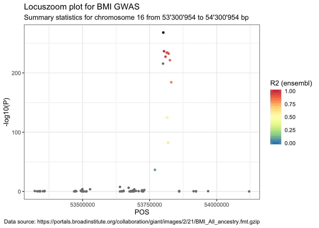

2. Solutions that work half-through

SNPsnap

SNPsnap: https://data.broadinstitute.org/mpg/snpsnap/database_download.html
uses a limited set of 1KG populations (EUR, EAS, WAFR).

API provided by sph.umich

API
uses limited set of 1KG populations (ALL, EUR)
see github issue

3. A solution that does not work

`rsnps::ld_search`

A perfect solution would have been the function ld_search from R package rsnps. It has arguments to choose the reference panel, the population, the distance from the focal SNP.

The problem is that it only uses old reference panels (HapMap and 1KG-phase1). Meaning, many newer reference panel populations are left out.

But the main problem is, that the broad institute has taken down the snap server that ld_search used to access (see github issue); hence ld_search is defunct.

Conclusion

The ldlink API with the LDproxy module seems the most perfect solution for now.

This will probably change with changing technology and larger reference panels.

Session Info

sessionInfo()

## R version 3.5.1 (2018-07-02)
## Platform: x86_64-apple-darwin15.6.0 (64-bit)
## Running under: macOS  10.14.5
## 
## Matrix products: default
## BLAS: /Library/Frameworks/R.framework/Versions/3.5/Resources/lib/libRblas.0.dylib
## LAPACK: /Library/Frameworks/R.framework/Versions/3.5/Resources/lib/libRlapack.dylib
## 
## locale:
## [1] en_US.UTF-8/en_US.UTF-8/en_US.UTF-8/C/en_US.UTF-8/en_US.UTF-8
## 
## attached base packages:
## [1] stats     graphics  grDevices utils     datasets  methods   base     
## 
## other attached packages:
##  [1] janitor_1.2.0      data.table_1.12.2  rsnps_0.3.2.9121  
##  [4] glue_1.3.1.9000    magrittr_1.5       xml2_1.2.0        
##  [7] jsonlite_1.6       httr_1.4.0         forcats_0.4.0.9000
## [10] stringr_1.4.0      dplyr_0.8.3.9000   purrr_0.3.2       
## [13] readr_1.3.1        tidyr_0.8.3.9000   tibble_2.1.3      
## [16] ggplot2_3.2.0.9000 tidyverse_1.2.1   
## 
## loaded via a namespace (and not attached):
##  [1] tidyselect_0.2.5 xfun_0.8         haven_2.1.1      lattice_0.20-38 
##  [5] colorspace_1.4-1 vctrs_0.2.0.9000 generics_0.0.2   htmltools_0.3.6 
##  [9] yaml_2.2.0       utf8_1.1.4       XML_3.98-1.20    rlang_0.4.0     
## [13] pillar_1.4.2     httpcode_0.2.0   withr_2.1.2      modelr_0.1.4    
## [17] readxl_1.3.1     plyr_1.8.4       munsell_0.5.0    blogdown_0.13   
## [21] gtable_0.3.0     cellranger_1.1.0 rvest_0.3.4      evaluate_0.14   
## [25] knitr_1.23       curl_3.3         fansi_0.4.0      triebeard_0.3.0 
## [29] urltools_1.7.3   broom_0.5.2      Rcpp_1.0.1       scales_1.0.0    
## [33] backports_1.1.4  hms_0.4.2        digest_0.6.20    stringi_1.4.3   
## [37] bookdown_0.11    grid_3.5.1       cli_1.1.0        tools_3.5.1     
## [41] lazyeval_0.2.2   crul_0.8.0       crayon_1.3.4     pkgconfig_2.0.2 
## [45] zeallot_0.1.0    ellipsis_0.2.0.1 lubridate_1.7.4  assertthat_0.2.1
## [49] rmarkdown_1.13   rstudioapi_0.10  R6_2.4.0         icon_0.1.0      
## [53] nlme_3.1-140     compiler_3.5.1

statistical genetics R data visualisation