ggGWAS reasoning
Sina Rüeger
2019-07-31
gggwas-reasoning.RmdWhy bother with ggplot2 extension for GWAS summary statistic data visualisations?
This vignette lays out the motivation why having a ggplot2 extension is needed. But it also discusses existing alternatives and ways to create a ggplot2-like Q-Q plot and Manhattanplot.
GWAS data visualisations
There are two main data visualisations1 that are done after the GWAS is run2:
Q-Q plot: checks the deviation of the P-value distribution from the uniform distribution.
Manhattan plot: shows the P-value or summary statistic distribution along the chomosomal position.


By M. Kamran Ikram et al - Ikram MK et al (2010) Four Novel Loci (19q13, 6q24, 12q24, and 5q14) Influence the Microcirculation In Vivo. PLoS Genet. 2010 Oct 28;6(10):e1001184. doi:10.1371/journal.pgen.1001184.g001, CC BY 2.5, Link
Alternatives
Both plotting types can be applied in R with various functions. Just to name a few, here are some links which have also served as inspiration:
-
qqman: R package for GWAS results: http://www.gettinggeneticsdone.com/2014/05/qqman-r-package-for-qq-and-manhattan-plots-for-gwas-results.html -
ggman: R package with ggplot2 wrapper with some neat hacks https://github.com/mkanai/ggman - Recipe to create Manhattanplot in R with
qqman,ggplot2andplotly: https://www.r-graph-gallery.com/wp-content/uploads/2018/02/Manhattan_plot_in_R.html - Recipe for QQplots in
lattice(for historical reasons) https://genome.sph.umich.edu/wiki/Code_Sample:_Generating_QQ_Plots_in_R - Fast QQplot implementation in
ramwaspackage: https://rdrr.io/bioc/ramwas/man/qqplotFast.html - DYI
ggplot2Manhattan plots: https://github.com/pcgoddard/Burchardlab_Tutorials/wiki/GGplot2-Manhattan-Plot-Function -
ggbiopackage, a toolkit for genomic data (plotGrandLinearis an implementation for a Manhattan plot, usesGRangesobjects, ggplot2 wrapper): https://bioconductor.org/packages/release/bioc/html/ggbio.html -
ggman, wrapper (but no ggplot2 extension) for Manhattan plots: https://github.com/drveera/ggman - https://www.gettinggeneticsdone.com/2010/07/qq-plots-of-p-values-in-r-using-base.html
An often used package is qqman, that has a function for Q-Q plots qqman::qq and Manhattan plots qqman::manhattan.
And there are various ggplot2 wrappers (ggbio, ggman), but not actual extensions.
Reasons
The problem is two fold:
- GWAS summary statistics usually contains around 1 mio of rows, so plotting becomes a lengthy process.
- All existing packages use the base plotting functions, making it difficult to apply any functionalities that
ggplot2can (e.g. facetting, colouring).
The idea is therefore to create a ggplot2 extension that would facilitate all this: 1) fast plotting (through hexagons and filtering) and 2) building ggplot2 geoms and stats.
By writing a ggplot2 extension, we can inherit lots of the default ggplot2 functionalities and shorten the input.
Ways of making a ggplot2-like Q-Q plot plot
Let’s say we have GWAS summary statistics for a number of SNPs. We call this data gwas.summarystats: for a number of SNPs listed by row, we know the SNP identifier (SNP) and the P-value (P).
SNP     P
rs3342  1e-2
rs83    1e-2
...     ...
For illustration purposes, we will use the summary statistics dataset GWAS.utils::giant.
library(GWAS.utils)
#skimr::skim(giant)
summary(giant)
#>       CHR             POS                SNP            Tested_Allele
#>  Min.   : 1.00   Min.   :   220149   Length:10000       Length:10000
#>  1st Qu.: 4.00   1st Qu.: 33810156   Class :character   Class :character
#>  Median : 8.00   Median : 71004162   Mode  :character   Mode  :character
#>  Mean   : 8.55   Mean   : 79743155
#>  3rd Qu.:12.00   3rd Qu.:114753146
#>  Max.   :22.00   Max.   :248476804
#>  Other_Allele       Freq_Tested_Allele_in_HRS      BETA
#>  Length:10000       Min.   :0.01023           Min.   :-4.980e-02
#>  Class :character   1st Qu.:0.19750           1st Qu.:-2.800e-03
#>  Mode  :character   Median :0.45710           Median :-1.000e-04
#>                     Mean   :0.48108           Mean   :-4.439e-05
#>                     3rd Qu.:0.75913           3rd Qu.: 2.600e-03
#>                     Max.   :0.98977           Max.   : 4.480e-02
#>        SE                 P                N
#>  Min.   :0.001600   Min.   :0.0000   Min.   :498178
#>  1st Qu.:0.001800   1st Qu.:0.0460   1st Qu.:680198
#>  Median :0.002100   Median :0.2600   Median :688732
#>  Mean   :0.002596   Mean   :0.3406   Mean   :683795
#>  3rd Qu.:0.002800   3rd Qu.:0.6000   3rd Qu.:691571
#>  Max.   :0.010600   Max.   :1.0000   Max.   :795594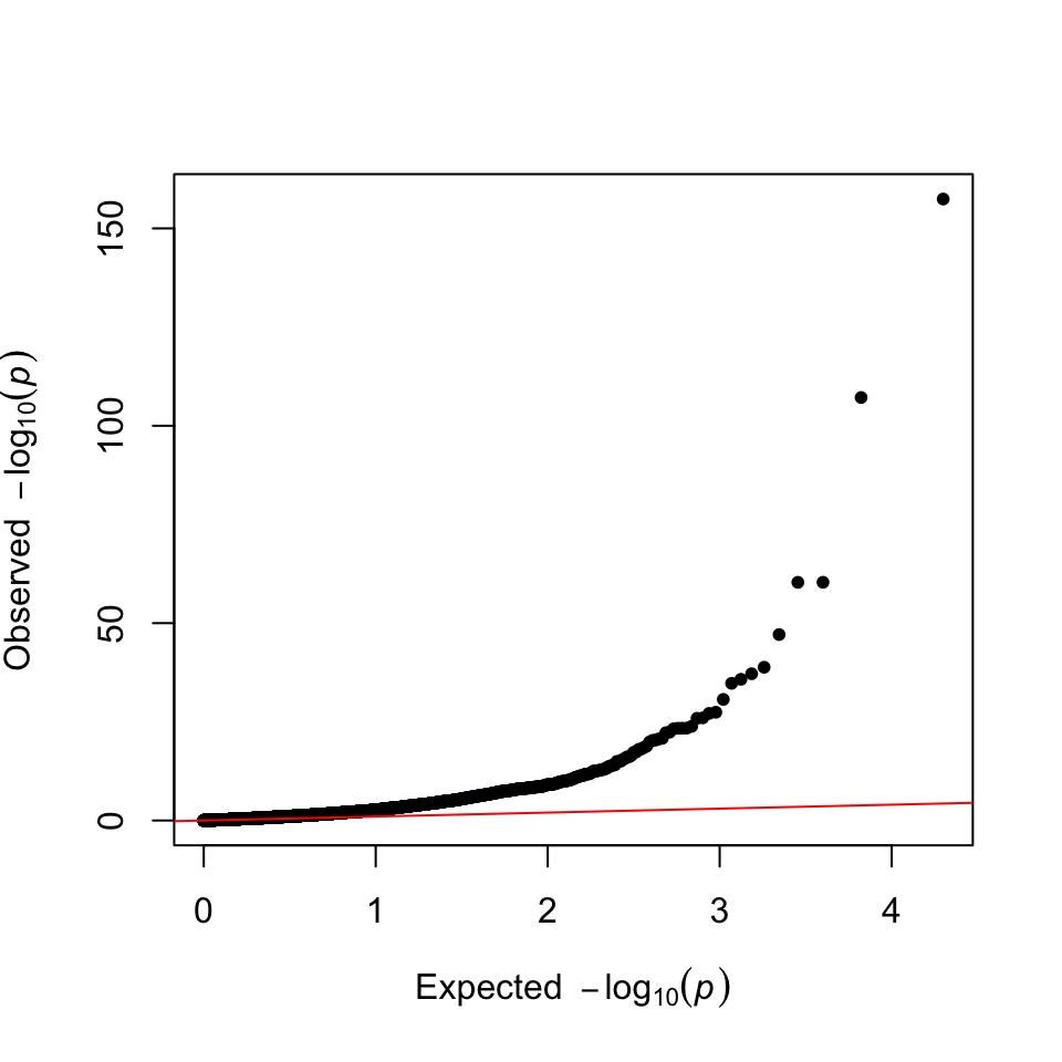
2. ggplot2::geom_qq
There is a geom_qq in ggplot2 that implements quantile-quantile plots. However, this is only useful, if we can transform the axes with -log10(). How to create custom made ggplot2 scales is explained here.
library(ggplot2)
theme_set(theme_bw())

## source:
(gg <- ggplot(data = giant) +
  geom_qq(aes(sample = P), distribution = stats::qunif)) +
    theme(aspect.ratio = 1)
# + scale_y_log10() + scale_x_log10()
# + coord_trans(x = "log10", y = "log10")

f_trans_mlog10 <- function(x) -log10(x)
f_trans_mlog10_inverse <- function(x) 10^(-x)

mlog10_trans <- scales::trans_new("-log10",
                                  transform = f_trans_mlog10,
                                  inverse = f_trans_mlog10_inverse)

gg +
  scale_y_continuous(trans = mlog10_trans) +
  scale_x_continuous(trans = mlog10_trans) +
  geom_abline(intercept = 0, slope = 1) +
  theme(aspect.ratio = 1)
3. ggplot2::geom_point
N <- nrow(giant)
expected <- (1:N) / N - 1 / (2 * N)
giant <- giant %>% dplyr::arrange(P) %>% dplyr::mutate(P_expected = expected)

ggplot(data = giant) +
  geom_point(aes(-log10(P_expected), -log10(P))) +
  geom_abline(intercept = 0, slope = 1) +
  theme(aspect.ratio = 1) +
  xlab(expression(Expected ~ ~-log[10](italic(p)))) + ## from qqman::qq
  ylab(expression(Observed ~ ~-log[10](italic(p)))) ## from qqman::qq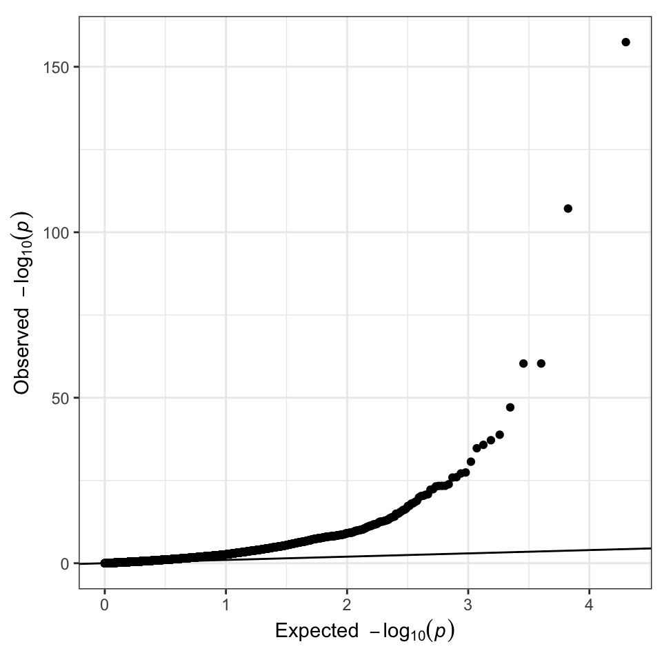
## or with the scale_y_continous feature
ggplot(data = giant) +
geom_point(aes(P_expected, P)) +
  scale_y_continuous(trans = mlog10_trans) +
  scale_x_continuous(trans = mlog10_trans) +
  geom_abline(intercept = 0, slope = 1) +
  theme(aspect.ratio = 1) #+ ## square shaped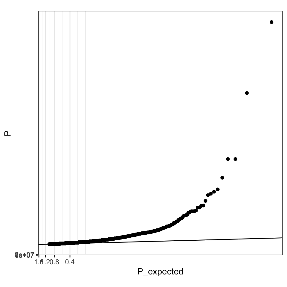
4. ggGWAS::geom_gwas_qq
ggplot(data = giant) + geom_gwas_qq(aes(y = P))
Here is a whishlist of what a geom_gwas_qq function should be able to do:
- include correct labels (expected as x-label and observed as y-label)
- make sure color, group, facetting all works
- allow for the
rasterversion (for faster plotting), hexbins (also for faster plotting) and Pvalue thresholding (removing the high Pvalue SNPs from the plot) - if time: implement genomic inflation factor representation
- while we are at it: plotting box should be squared (
theme(aspect.ratio = 1))
Ways of making a ggplot2-like Manhattan plot
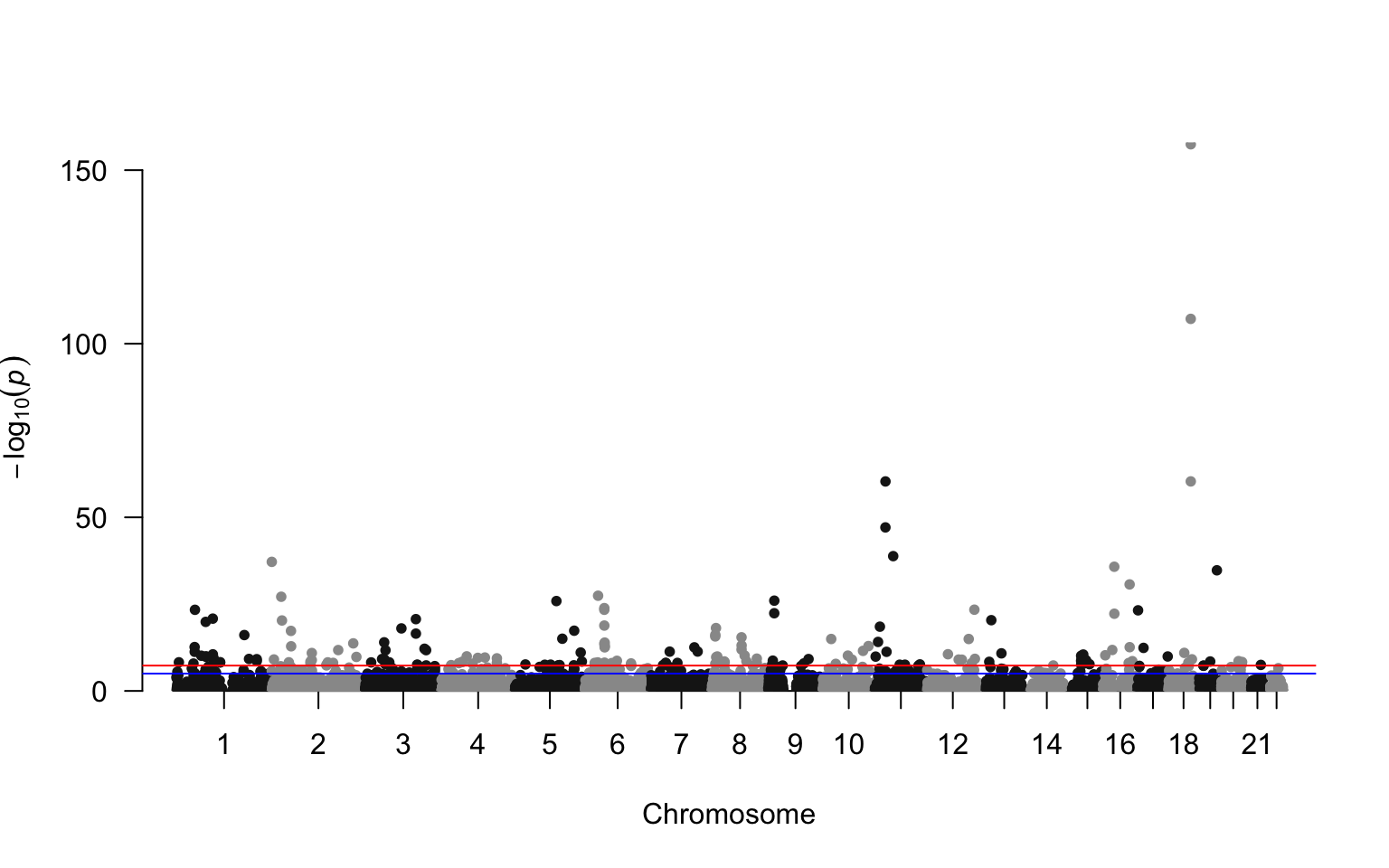
2. ggplot2::geom_point
## computing new x axis
giant <- giant %>% dplyr::arrange(CHR, POS) %>% dplyr::mutate(tmp = 1, cumsum.tmp = cumsum(tmp))

## calculating x axis location for chromosome label
med.dat <- giant %>% dplyr::group_by(CHR) %>% dplyr::summarise(median.x = median(cumsum.tmp))

ggplot(data = giant) +
  geom_point(aes(x = cumsum.tmp, y = -log10(P), color = CHR %%2 == 0)) + ## create alternate coloring
  geom_hline(yintercept = -log10(5e-8)) + ## add horizontal line
  scale_x_continuous(breaks = med.dat$median.x, labels = med.dat$CHR) + ## add new x labels
  guides(colour=FALSE) +  ## remove legend
  xlab("Chromosome") +
  ylab(expression(-log[10](italic(p)))) + ## y label from qqman::qq
  scale_color_manual(values = c(gray(0.5), gray(0))) ## instead of colors, go for gray
3. ggGWAS::geom_gwas_manhattan
ggplot(data = giant) + geom_gwas_manhattan(aes(pos = POS, chr = CHR, y = -log10(P)))
Here is a whishlist of what a geom_gwas_manhattan function should be able to do:
- x axis spacing with space between chromosome and spaced as with position
- include correct y axis labels
- make sure color, group, facetting all works
- allow for the
rasterversion (for faster plotting) and Pvalue thresholding (removing the high Pvalue SNPs from the plot) - implement coloring (two alternating colors)
Misc
Testing
How to test plots?
One option is, to compare ggplot2 object data. In the example below, we are comparing two ggplot2 outputs, one created with qplot and one with ggplot.
gg1 <- qplot(Sepal.Length, Petal.Length, data = iris)
gg2 <- ggplot(data = iris) + geom_point(aes(Sepal.Length, Petal.Length))
identical(gg1$data, gg2$data)
We can apply this to our package by creating the qqplot and manhattanplots manually by hand, and then comparing the to the function outputs.
Another option is to use https://github.com/lionel-/vdiffr